A* Algorithm In AI

A* (pronounced “A-star”) algorithm! If you’re new to computer science, artificial intelligence, or just curious about how computers find the shortest path in games like GPS navigation or video games, you’re in the right place. We’ll break down everything about A* in simple, easy-to-understand language. No prior knowledge is required—we’ll start from the basics and build up step by step.

By the end of this read, you’ll understand what A* is, how it works, why it’s powerful, and even see a real-world example with code. Think of this as your friendly roadmap (pun intended) to one of the most popular pathfinding algorithms out there. Let’s dive in!

What is the A* Algorithm? An Introduction

Imagine you’re trying to get from your home to a friend’s house in a busy city. You could take a random path, but that’s inefficient. Or you could use a map app that suggests the quickest route, avoiding traffic and dead ends. That’s essentially what the A* algorithm does in the digital world—it’s a smart way for computers to find the shortest or most efficient path from a starting point to a goal in a graph or map.

A* was developed in 1968 by Peter Hart, Nils Nilsson, and Bertram Raphael as an extension of Dijkstra’s algorithm. It’s widely used in fields like robotics, video games (e.g., in games like The Sims or StarCraft for character movement), GPS systems, and even puzzle solvers like the 8-puzzle or Rubik’s Cube.

Why is it called A*? The “A” stands for “algorithm,” and the asterisk (*) hints at it being the “best” or optimal version in its class. It’s a heuristic search algorithm, meaning it uses educated guesses (heuristics) to speed things up without sacrificing accuracy.

In simple terms:

Graph: A network of points (nodes) connected by lines (edges), like a city grid.
Pathfinding: Finding a way from node A to node Z.
A* shines because it’s efficient (fast) and optimal (finds the best path) under certain conditions.

The Basics: Understanding Graphs and Search Algorithms

Before we jump into A*, let’s cover some groundwork. Skip ahead if you’re familiar!

What is a Graph?

A graph is like a web of connections:

Nodes (Vertices): Points, e.g., intersections in a city.
Edges: Connections between nodes, which can have weights (costs), like distance or time.
Types: Directed (one-way streets) or undirected (two-way).

For pathfinding, we often use grids (like a chessboard) where each square is a node, and you can move up, down, left, right.

Common Search Algorithms Before A*

To appreciate A*, know its predecessors:

Breadth-First Search (BFS): Explores level by level, like ripples in a pond. Great for unweighted graphs but slow for large ones.
Depth-First Search (DFS): Dives deep into one path before backtracking. Can get stuck in long dead ends.
Dijkstra’s Algorithm: Like BFS but for weighted graphs. It always finds the shortest path by exploring the cheapest paths first. However, it’s “blind”—it doesn’t guess where the goal is, so it can waste time exploring irrelevant areas.
Greedy Best-First Search: Uses a heuristic (guess) to always pick the path that seems closest to the goal. Fast but not always optimal—it might miss shorter paths.

A* combines the best of Dijkstra’s (guaranteed optimality) and Greedy (speed via heuristics).

How Does A* Work? The Core Mechanics

A* maintains two lists:

Open Set: Nodes to explore (starts with the start node).
Closed Set: Nodes already explored.

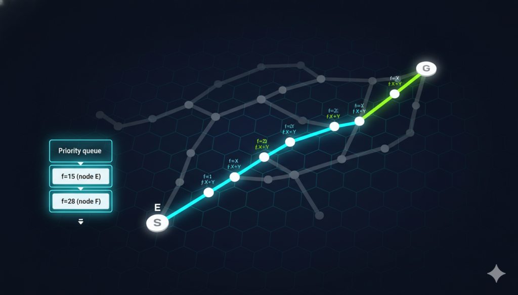
It uses a priority queue for the open set, sorted by a score called f(n), which estimates the total cost of the path through node n.

The Key Formulas

A* evaluates nodes using three values:

g(n): The exact cost from the start node to the current node n. (Like the distance traveled so far.)
h(n): The heuristic estimate of the cost from n to the goal. (A “best guess” of remaining distance, e.g., straight-line distance in a map.)
f(n) = g(n) + h(n): The total estimated cost. A* always picks the node with the lowest f(n) to explore next.

The heuristic h(n) is what makes A* “informed” and faster than Dijkstra’s (which is like A* with h(n)=0).

Step-by-Step Algorithm

Here’s how A* runs:

Initialize:
- Set start node’s g=0, h=heuristic to goal, f=g+h.
- Add start to open set.
- Create a “came_from” map to reconstruct the path later.
Loop While Open Set Isn’t Empty:
- Pick the node with the lowest f(n) from open set (call it current).
- If current is the goal, reconstruct and return the path!
- Move current to closed set.
- For each neighbor of current:
  - If neighbor is in closed set or blocked (e.g., a wall), skip.
  - Calculate tentative_g = g(current) + distance(current to neighbor).
  - If neighbor not in open set or tentative_g < g(neighbor):
    - Update came_from[neighbor] = current.
    - Update g(neighbor) = tentative_g.
    - Update h(neighbor) = heuristic(neighbor to goal).
    - Update f(neighbor) = g + h.
    - Add/update neighbor in open set.
If Open Set Empties Without Finding Goal: No path exists.

It’s like a smart explorer: It balances actual progress (g) with optimistic guesses (h) to focus on promising paths.

To visualize, imagine a grid where you’re finding a path from top-left to bottom-right, avoiding obstacles. A* would expand fewer nodes than Dijkstra’s by prioritizing directions toward the goal.

(Above: A typical diagram showing A* in action on a grid, with nodes colored by their f-scores.)

Heuristics: The Secret Sauce of A*

The heuristic h(n) is crucial—it’s your “gut feeling” about how far the goal is.

Good Heuristics

Admissible: Never overestimates the true cost (h(n) ≤ true cost). This ensures A* finds the optimal path.
Consistent (Monotonic): For every node n and successor m, h(n) ≤ cost(n to m) + h(m). This makes A* even more efficient (no need to re-expand nodes).

Common heuristics for grids:

Manhattan Distance: |x2 – x1| + |y2 – y1| (for 4-directional movement, like city blocks).
Euclidean Distance: sqrt((x2 – x1)^2 + (y2 – y1)^2) (for any direction, like straight lines).
Octile Distance: For 8-directional movement, combining Manhattan and diagonal costs.

If your heuristic is inadmissible (overestimates), A* might find a suboptimal path but faster. For optimality, stick to admissible ones.

Example: In a map, using straight-line distance (Euclidean) is admissible because the real path can’t be shorter than a straight line.

(Above: Illustration of different heuristics in pathfinding.)

A Real Example: A* on a Simple Grid

Let’s apply A* to a 5×5 grid. Start at (0,0), goal at (4,4). Obstacles at (2,1), (2,2), (2,3). Use Manhattan heuristic.

Start: g=0, h=8 (4+4), f=8.
Explore neighbors: Right (1,0): g=1, h=7, f=8. Down (0,1): g=1, h=7, f=8.
Pick one, say (1,0). Explore its neighbors, and so on.
A* will snake around the obstacles, always choosing low f(n).

For a hands-on feel, here’s a simple Python implementation. I’ll explain the code, then show a run.

import heapq  # For priority queue

def a_star(grid, start, goal):
    def heuristic(a, b):
        return abs(a[0] - b[0]) + abs(a[1] - b[1])  # Manhattan

    rows, cols = len(grid), len(grid[0])
    open_set = []
    heapq.heappush(open_set, (0, start))  # (f, position)
    came_from = {}
    g_score = {start: 0}
    f_score = {start: heuristic(start, goal)}

    directions = [(0,1), (1,0), (0,-1), (-1,0)]  # Right, down, left, up

    while open_set:
        current_f, current = heapq.heappop(open_set)
        if current == goal:
            path = []
            while current in came_from:
                path.append(current)
                current = came_from[current]
            path.append(start)
            return path[::-1]  # Reverse to start->goal

        for dx, dy in directions:
            neighbor = (current[0] + dx, current[1] + dy)
            if 0 <= neighbor[0] < rows and 0 <= neighbor[1] < cols and grid[neighbor[0]][neighbor[1]] == 0:  # 0 = walkable
                tentative_g = g_score[current] + 1
                if neighbor not in g_score or tentative_g < g_score[neighbor]:
                    came_from[neighbor] = current
                    g_score[neighbor] = tentative_g
                    f_score[neighbor] = tentative_g + heuristic(neighbor, goal)
                    heapq.heappush(open_set, (f_score[neighbor], neighbor))

    return None  # No path

# Example grid: 0=empty, 1=obstacle
grid = [
    [0, 0, 0, 0, 0],
    [0, 0, 1, 0, 0],
    [0, 0, 1, 0, 0],
    [0, 0, 1, 0, 0],
    [0, 0, 0, 0, 0]
]
start = (0, 0)
goal = (4, 4)
path = a_star(grid, start, goal)
print("Path:", path)

Running this (mentally or in code): Path might be [(0,0), (0,1), (0,2), (0,3), (0,4), (1,4), (2,4), (3,4), (4,4)] or similar, avoiding the column of obstacles.

This code uses a priority queue (heapq) to always pick the lowest f. Time complexity: O(b^d) in worst case, but heuristics make it much better (b=branching factor, d=depth).

Advantages and Disadvantages of A*

Pros:

Optimal: With admissible heuristic, guarantees shortest path.
Efficient: Explores fewer nodes than uninformed searches.
Flexible: Works on any graph, with various heuristics.
Complete: Will find a path if one exists.

Cons:

Memory Usage: Open/closed sets can get large in big graphs (mitigated by variants like IDA*).
Heuristic Dependency: Bad heuristic = poor performance.
Not Real-Time: For massive graphs, it might be slow without optimizations.

Compared to others:

Faster than Dijkstra’s in practice.
More reliable than Greedy (which can be suboptimal).

Real-World Applications

A* isn’t just theory—it’s everywhere:

Video Games: Pathfinding for NPCs (non-player characters) in games like Path of Exile or Minecraft.
Robotics: Robots navigating warehouses (e.g., Amazon bots).
GPS and Maps: Google Maps uses similar ideas for route planning.
AI Planning: In puzzles, network routing, or even protein folding in biology.
Variants: Like D* for dynamic environments (changing maps).

In 2026, with AI advancements, A* is integrated into self-driving cars and drone navigation for obstacle avoidance.

Common Pitfalls and Tips

Ties in f(n): Break ties with h(n) or g(n) to optimize.
Weighted Edges: Adjust distances accordingly.
Infinite Loops: Ensure closed set prevents re-visits.
Debugging: Print g/h/f values to understand behavior.

If implementing, test on small grids first!

Conclusion: Why Learn A*?

A* is a cornerstone of AI pathfinding—elegant, powerful, and practical. Whether you’re a student, developer, or hobbyist, understanding A* opens doors to more advanced topics like machine learning or game dev. It’s like learning to drive: Once you get it, you can navigate complex problems with ease.

If you want to experiment, try coding it yourself or use libraries like NetworkX in Python. Questions? Drop a comment below!

Thanks for reading—happy pathfinding! 🚀

(This blog is for educational purposes. Code examples are simplified; real implementations may vary.)