Search Space Control is one of the most important and scoring topics in Artificial Intelligence, especially from academic and exam perspectives. Almost every AI problem—whether it is game playing, path finding, planning, or optimization—requires searching through a large number of possibilities. The main challenge is how to search efficiently, and that is exactly where search space control comes into play.
In this explanation, we will go from very basic concepts to advanced techniques, with intuition, examples, and structured theory.
In AI, many problems are framed as search problems, where you start from an initial situation and aim to reach a goal by applying actions. The “search space” (often called state space) is the collection of all possible configurations or states. Controlling this space means using strategies to explore it smartly, avoiding unnecessary paths and focusing on promising ones. Think of it like exploring a massive maze: without a plan, you’d wander forever, but with guides (like heuristics), you can find the exit faster.
This blog will break it down step by step, from basics to advanced techniques, with examples, algorithms, and visuals. By the end, you’ll understand how AI systems “think” through problems like chess moves or route planning. Let’s get started!
What is State Space in AI?
At its core, AI search involves modeling a problem as a state space, which is a graph where:
- Nodes represent states (specific configurations of the problem).
- Edges represent actions or transitions that move you from one state to another.
For instance, in a chess game, a state could be the current board position, and an action is moving a piece.
Key components include:
- Initial State: Where you begin (e.g., the starting board in a puzzle).
- Goal State: The target (e.g., solved puzzle).
- Actions: Possible moves (e.g., slide a tile left).
- Transition Model: Rules for how actions change states.
- Path Cost: A measure of effort, like the number of moves.
The state space can be enormous— for a simple 3×3 puzzle, there are over 180,000 reachable states! Without control, exploring everything (exhaustive search) is impractical due to exponential growth: if each state has b possible actions (branching factor) and the solution is at depth d, you might check up to b^d states. For b=10 and d=5, that’s 100,000 states—imagine deeper problems!
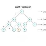
To visualize, here’s a diagram showing a typical state space as a graph:
The Need for Search Space Control
Why control the search space? Uncontrolled search leads to the combinatorial explosion, where the number of possibilities grows too fast for computers to handle. Control strategies decide which paths to explore first, prune dead ends, and use knowledge to guide the process.
Control is implemented through:
- Data Structures: Stacks for depth-first, queues for breadth-first, priority queues for best-first.
- Backtracking: Retracing steps when a path fails.
- Loop Detection: Using a “closed list” to avoid revisiting states.
- Heuristics: Estimates to prioritize promising paths.
These strategies fall into two main categories: uninformed (blind) and informed (heuristic-guided). Advanced methods like production systems add modularity for complex problems.
Uninformed Search Strategies
Uninformed strategies explore without extra problem knowledge—they’re systematic but can be inefficient.
Breadth-First Search (BFS)
BFS explores level by level, like ripples in a pond. It uses a queue: add the initial state, expand its children, then their children, and so on.
Algorithm Steps:
- Enqueue the initial state.
- While queue not empty:
- Dequeue a state.
- If it’s the goal, return the path.
- Else, generate successors, enqueue unvisited ones.
- Use a set for visited states to avoid cycles.
Pros: Complete (finds a solution if exists); optimal for equal-cost actions (shortest path). Cons: High memory (stores all nodes at current level); time O(b^d).
Ideal for finding the shortest path in unweighted graphs, like simple puzzles.
Depth-First Search (DFS)
DFS dives deep into one path before trying siblings, using a stack (or recursion).
Algorithm (Recursive Version):
function DFS(node, goal, path, visited):
    if node == goal:
        return path + [node]
    visited.add(node)
    for child in generate_children(node):
        if child not in visited:
            result = DFS(child, goal, path + [node], visited)
            if result:
                return result
return NonePros: Low memory (only current path). Cons: Not complete without depth limits (can loop infinitely); not optimal.
Useful for deep spaces where solutions are far down one branch.
Other uninformed: Uniform Cost Search (like BFS but with costs), Depth-Limited Search (DFS with max depth).
Informed Search Strategies
Informed strategies use heuristics—rules of thumb estimating distance to the goal—to focus on promising areas.
Greedy Best-First Search
Expands the “best” node first based on heuristic h(n) (estimated cost to goal).
Pros: Faster than uninformed. Cons: Not optimal; can get stuck in local optima.
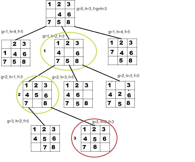
A* Search
The gold standard: Combines path cost g(n) (from start) with h(n) in f(n) = g(n) + h(n). Uses priority queue.
Algorithm:
- Priority queue sorted by f(n).
- Expand lowest f(n) node.
- Stop at goal.
For optimality, h(n) must be admissible (never overestimate) and consistent (monotonic).
Pros: Complete and optimal with good heuristic. Cons: Still memory-intensive.
Example heuristic for puzzles: Manhattan distance (sum of tile displacements).
Advanced Control Techniques
Beyond basic algorithms, AI uses structured systems for control.
Recursion-Based Search
Implements DFS via recursion: Each call explores a child, backtracks on failure. Efficient for tree-like spaces but risks stack overflow in deep searches.
Pattern-Directed Search
Uses logic (e.g., predicates) to match patterns and unify variables. Basis for languages like Prolog. Great for goal-directed inference.
Production Systems
A modular framework:
- Rules: If condition, then action.
- Working Memory: Current state.
- Cycle: Match rules, select/fire one, update memory.
Control can be data-driven (forward from facts) or goal-driven (backward from goal). Examples include expert systems.
Advantages: Separates knowledge from control; easy to explain reasoning.
Blackboard Architecture
For collaborative solving: Multiple “knowledge sources” post to a shared blackboard, coordinating complex tasks like speech recognition.
Real-World Examples
Let’s apply these concepts.
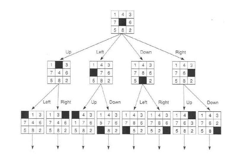
The 8-Puzzle Problem
A 3×3 grid with tiles 1-8 and a blank. Goal: Order them with blank at bottom-right.
State: Grid array. Actions: Move blank up/down/left/right.
Use BFS for shortest solution or A* with heuristic (e.g., misplaced tiles).
Here’s an example initial and goal state:
Python BFS code (simplified from earlier):
from collections import deque
import numpy as np

def bfs(initial, goal):
    queue = deque([(initial, [])])
    visited = set([tuple(initial.flatten())])

    while queue:
        state, path = queue.popleft()
        if np.array_equal(state, goal):
            return path + [state]

        blank = tuple(np.argwhere(state == 0)[0])
        moves = [(-1, 0), (1, 0), (0, -1), (0, 1)]

        for dx, dy in moves:
            nx, ny = blank[0] + dx, blank[1] + dy
            if 0 <= nx < 3 and 0 <= ny < 3:
                new_state = state.copy()
                new_state[blank], new_state[(nx, ny)] = new_state[(nx, ny)], new_state[blank]
                new_tuple = tuple(new_state.flatten())
                if new_tuple not in visited:
                    visited.add(new_tuple)
                    queue.append((new_state, path + [state]))
    return None
To solve: Call with np arrays for initial/goal.
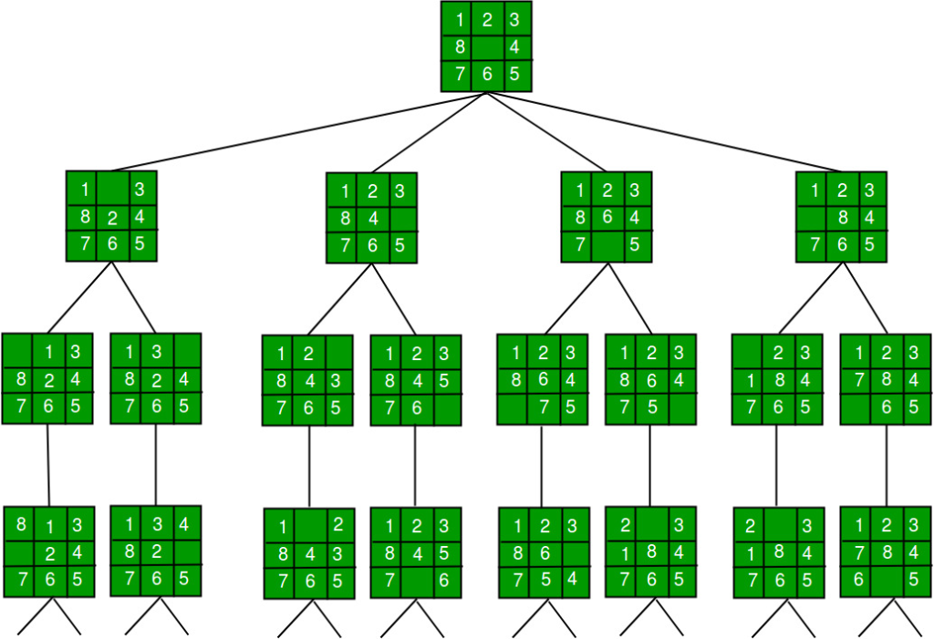
Another view of state transitions:
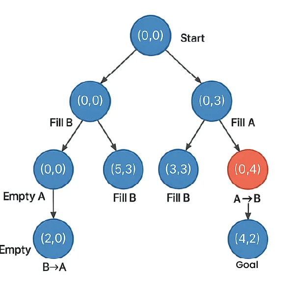
Water Jug Problem
The Water Jug Problem is one of the most famous classical problems in Artificial Intelligence and problem-solving. It is mainly used to explain state space search, problem formulation, and search algorithms like BFS and DFS.
I’ll explain this from absolute basics to advanced AI concepts, step by step.
The Water Jug Problem is a puzzle where you are given:
- Two jugs with fixed capacities
- An unlimited water supply
- No measuring marks on the jugs
Goal: Measure exactly a target amount of water using only allowed operations.
Classic Problem Statement
You are given:
- Jug A with capacity 4 liters
- Jug B with capacity 3 liters
- You must measure 2 liters of water
Allowed Operations:
- Fill a jug completely
- Empty a jug completely
- Pour water from one jug to another until:
- the source jug is empty, or
- the destination jug is full
You cannot:
- Measure water directly
- Spill water except by emptying a jug
The problem can be solved using search algorithms.
Breadth First Search (BFS)
- Explores level by level
- Guarantees shortest solution
- Most commonly used for Water Jug Problem
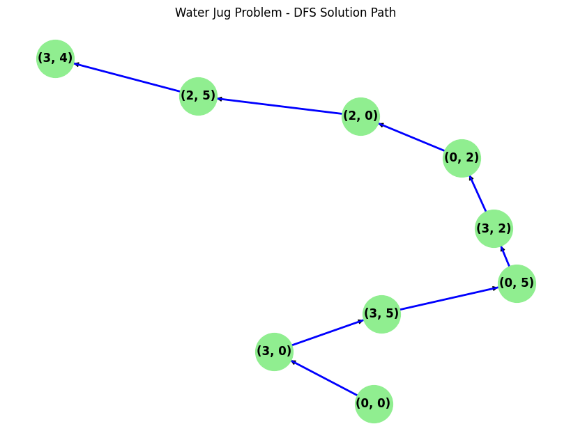
Depth First Search (DFS)
- Goes deep first
- May get stuck in loops
- Does not guarantee optimal solution
State space tree example:
DFS traversal diagram:
Knight’s Tour
On a chessboard, find a path where a knight visits every square once. Use pattern-directed search with rules for moves.
Challenges and Optimizations
- Challenges: Memory limits, time explosion, poor heuristics.
- Optimizations: Pruning (e.g., alpha-beta in games), dimensionality reduction, hybrid strategies.
In machine learning, similar ideas apply to hyperparameter search or reinforcement learning.
Conclusion
Search space control is the backbone of AI problem-solving, turning chaotic possibilities into efficient paths. From BFS’s thoroughness to A*’s smarts and production systems’ modularity, these techniques empower AI in games, robotics, and more. As a student, experiment with code—try solving the 8-puzzle yourself!
Remember, AI is about smart exploration, not brute force. Keep learning, and you’ll master controlling the vast spaces of intelligence.
Sources and further reading are cited inline for credibility. Happy studying!